Alan Turing and Computability

Yesterday (June 23), would have been the 100th birthday of Alan Turing, the mathematician who was one of the founders of modern computer science – indeed he is often considered to be the “father of computer science.”

In the 1920s and 1930s, much attention in the mathematics was on the subject of “computable numbers” and finding automatic systems for proving mathematical statements.   Based on a series of problems stated by David Hilbert, the mathematician Kurt Gödel ultimately proved that this not possible.  Essentially, there is no formal mathematical system that can decide the truth or falsehood of all mathematical statements.   This is quite profound and simple to state, but Gödel’s mathematics is cryptic and at some times impenetrable.   By contrast, Alan Turing’s formulation of the mathematics as a simple device is quite accessible and laid the groundwork for the positive use of Gödel’s results.  Sure, we cannot solve all mathematical problems computationally, but we can do quite a lot with the right tools.  The Turing Machine is one of the simpler of such tools.


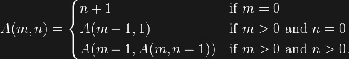
A Turing Machine consists of a tape, or an infinite sequence of cells, each of which contains a symbol that can be read or written.  There is a head, which (much like the head on a tape recorder) moves along the tape and is always positioned at one cell.  The state register contains one or more states of the machine.  Finally, the transition table contains a series of instructions of the form qiaj→qi1aj1dk where q is a state, a is a symbol, and d is a number of cells to move the head left or right along the tape (including not moving it at all).  So, if the machine is at a given state qi and the head is over a symbol aj, switch to state qi1, write the symbol aj1 at the head, and move the head dk positions to the left or right.

The description of the Turing Machine is very mechanical, which makes it a bit easier to understand.  But it is nonetheless a formal mathematical model.  It was used to demonstrate that the “halting problem”, the ability of such a machine to determine if any set of states and transitions will stop or repeat forever, is not solvable.  This remains today, one of the great unsolvable problems in computer science.

About the same time as Turing published his results, American mathematician Alonzo Church published an equivalent result using lambda calculus, a system I personally find more intuitive and elegant because of its basis in functions and algebraic-like expressions (it will be the subject of a future article).  But Turing’s work has been more prominent both in mainstream computer science and in the culture at large, with computer designs and languages being described as “Turing complete”.  And then there is the “Turing Test” for evaluating artificial intelligence systems.  So far, no system has ever passed the test.

During this centennial, especially coming as it does during Pride Weekend in much of the United States, there has been much written about Turing’s homosexuality and his being convicted for homosexual activity that was then illegal in the UK and stripped of his security clearance.  This is a very sad statement on the time in which he lived, that someone who was both one of the most influential mathematicians in a growing field of computation and a hero of World War II for is code-breaking exploits was treated in such a mean and undignified way.  There was also much written about the mysterious circumstances of his death – long considered a suicide, a recent BBC article on the centennial suggests otherwise.  You can read for yourself here.  As for us at CatSynth, we prefer to focus on his achievements.

Google honored Turing yesterday with one of their trademark “Google Doodles” in which they implemented a functioning Turing Machine.


Ackermann’s Function and “Really Big Numbers”

Today we return to to the topic of mathematics with a look at Ackermann’s Function. Anyone who has studied computer science has probably encountered this function (though I’m sure many have gone on to forget it). It is most commonly defined as follows:

This is actually a variant of Wilhelm Ackermann’s original function, often called the Ackermann–Péter function. It is quite a simple function to define and to trace, and it is very easy to implement in just about any programming language, including Python:

def ackermann(m, n):
  if m == 0:
    return n + 1
  elif n == 0:
    return ackermann(m - 1, 1)
  else:
    return ackermann(m - 1, ackermann(m, n - 1))

However, its complexity (in terms of run-time and memory) grows quite quickly. As such, it is often used as an exercise in teaching students more complex forms of recursion, and also as a test case in compiler development for optimizing recursion. It also has some interesting mathematical properties for particular values of m:

The numbers in the case of A(4,n) are quite large. Indeed, one could describe Ackermann’s function as “computing really really large numbers really really slowly.” Although the numbers grow quickly, the function is really just doing subtraction and recursion. We can take advantage of the properties described above, however, to make some shortcuts that yield a much more efficient function.

def ackermann(m, n):
  while m >= 4:
    if n == 0:
      n = 1
    else:
      n = ackermann(m, n - 1)
    m -= 1
  if m == 3:
    return 2 ** ( n + 3) - 3
  elif m == 2:
    return 2 * n + 3
  elif m == 1:
    return n + 2
  else: # m == 0
    return n + 1

With this version computing A(m,n) for m≤3 becomes trivial. And this makes computations for m≥4 possible. Or at least A(4,2), which we can actually run in python to reveal the 19,000 digit answer.

You can see the full value on this page. Computing A(4,3) is infeasible. Even with the optimizations, most computers will run out of memory trying to compute this value. But one can still reason about these rather large numbers. Let us move from the more common function we have been using to Ackermann’s original version:

This version has three arguments instead of two, and on the surface it may seem a bit more complicated. However, different values of the third argument p yield very familiar operations.


Again, this function is a rather inefficient way to compute addition, multiplication and exponentiation, but it is an interesting way to reason about them and extrapolate to other more exotic operations. For example, if we take p to be 3, we get the following operation.

Just as m x n is adding m to itself n times, and exponentiation mn is multiplying m by itself n times, this new operation (sometimes called tetration) is the next level: exponentiating m by itself n times.

Such an operation grows so fast as to be uncomparable to exponential growth. It grows even too fast to compare to the gamma function which have explored on CatSynth in the past. This series of ever higher-order operations is often noted with an arrow, called Knuth’s up-arrow notation after legendary computer scientist Donald Knuth.

Using this notation, we can define as sequence of numbers, called Akermann Numbers, where each is an ever higher-order operation of the element applied to itself.

  • 1↑1 = 11 = 1,
  • 2↑↑2 = 2↑2 = 22 = 4,
  • 3↑↑↑3 = 3↑↑3↑↑3 = 3↑↑(3↑3↑3) = 

Even just the 4th number is this sequence is so large that we can’t even easily notate it with exponents. So forget about the 5th number in sequence. But a question that interests me is what about interpolating with real numbers. What is the 1 1/2th Ackermann number? That question, if it even has an answer, will have to wait for another time.

Dissertation now (back) online

I have finally reposted my doctoral dissertation, this time in HTML format as well as PDF. The title is Perceptual Scheduling in Real-time Music and Audio Applications. I propose an algorithm for improving computational performance of expensive synthesis techniques, such as additive synthesis and resonance modeling that preserves audio quality, and measured both the improved CPU performance and the perceptual quality as measured by expert listeners in controlled experiments.

I think this actually a good time to review and reflect upon this work. Five years have passed since I graduated from UC Berkeley with my PhD. I probably have the only doctoral dissertation in Computer Science that includes James Brown as a citation. While I enjoyed working on the dissertation, including the formal experiments, the work I do now developing music software (and then using for my own composition and performance) is really a better match for who I am.

As discussed in an earlier post, I have had a sometimes challenging relationship with academic science. I have the technical and analytical “chops”, but I am too much of a creator and a romantic to find personal meaning and reward in rigorous experiments and analysis of data. I love the aesthetic appeal of science and mathematics, and especially look for unusal and serendipitous connections rather standard incremental results. Simply put, I am an artist, not a scientist, even when I'm working on software engineering projects.