The Fundamental Theorem of Arithmetic

It is not uncommon to hear operations on numbers, even the computations carried out in modern computers, as “mere arithmetic.” But arithmetic is hardly simple or obvious when one gets down to the fundamentals and realizes the structure that must be present in our number system in order for it to work they way we intuitively think it should work. Thus, today we consider the Fundamental Theorem of Arithmetic.

Every positive integer (except the number 1) can be represented in exactly one way apart from rearrangement as a product of one or more primes.

Thus every integer has a canonical representation as a product of powers of primes:

where p1 < p2 < … < pk are primes and the αi are positive integers; 1 is represented by the empty product. As example 12 = 22 × 3, and 666 = 2 × 32 × 37. Fairly familiar stuff for anyone who paid attention during grade school and secondary school math classes. But the theorem itself is not self-evident, it is something that had to be proven true in order for our everyday arithmetic to hold. A good article on why the theorem is not obvious can be found here. It also has implications beyond the natural numbers. If we extend the canonical representation to allow both positive and negative values for ai, we get the set of positive rational numbers (fractions), for which the theorem still holds. It can also be generalized to more exotic constructions, such as Gaussian Integers. Gaussian integers, often denoted ℤ[i] are complex numbers a + bi where i is the square root of -1, and a and b are integers. It can be shown that the fundamental theorem of arithmetic holds for Gaussian integers, and that there is a definite set of “Gaussian primes” just as there are prime numbers. But while plotting the prime numbers and looking for visual patterns is an exercise in frustration, the rotational nature of complex numbers (which we have discussed in a previous article) causes the Gaussian primes to fall into a visually interesting radial pattern:

With all the important and sometimes confounding properties of primes, having ways to visualize them is always intriguing.

Any mathematical construct (specifically, a “domain”) that obeys the fundamental theorem of arithmetic is known as a Euclidean Domain. (Note that this has very little to do with Euclidean spaces or the other uses of the term in geometry.) We can observe many more Euclidean domains, such as generalizing Guassian integers to other roots of 1. If we use the cube roots of 1, for example (yes, 1 has three cube roots), we get the set of Eisenstein Integers: numbers of the form a + bω, where a and b are integers and:

Like Gaussian primes, Eisenstein primes have a distinctive radial pattern when viewed on the complex plane. Whereas Guassian primes divide into quadrants, Eisenstein primes form a hexagonal pattern.

Note that while the generalization works for square roots of -1, cube roots of 1, etc., it doesn’t necessarily work for all roots of 1. Some of those sets will not form Euclidean domains.

We can also look beyond numbers to other mathematical entities that form Euclidean domains. One such example can be found in knot theory, which we discussed in an article a few years ago. Knots can be expressed as unique combinations of prime knots:

From here we can consider the implications for music of the Euclidean domains, the accompanying Euclidean algorithm for computing greatest common divisors in any of these domains. But that will be left as an exercise for another day.

Eye to Eye: Imaginary Exponentiation

The term “imaginary number” is an unfortunate one. It makes these numbers seem strange and separate from more familiar “real” numbers, when in fact there is very little difference. I prefer the term complex numbers that encompasses the closed set of all real and imaginary numbers with the usual arithmetic operators. Recall that the imaginary numbers are numbers that are less then zero when squared, with the imaginary constant i representing the square root of -1:

i 2 = -1

One can add, subtract, multiply and divide with it just like other numbers. One can not only square it to get -1, but also take its square root, which turns out to be another complex number.

 i  = 2/2 + i 2/2

But what about raising i to the ith power?

Surely, that must be some sort of weird “very imaginary” number, right? But in fact, it is just a real number, approximately 0.2078796…

The same mechanism that allows us to take the square root of i can be used to explain why ii is real. Just as real numbers can be visualized on the familiar number line, complex numbers can be represented by a plane where the horizontal axis represents real numbers and the vertical axis represents imaginary numbers.

Any complex number x + yi can also be expressed with an angle and a radius: rcosθ+risinθ. Using the angular representation on the plane, we can then visualize any exponentiation operation (take the square, the square root, etc.) as a rotation around the origin.

Squaring a number means doubling the angle. Taking the square root means cutting the angle in half. The imaginary constant i has a radius of 1 and an angle of 90 degrees (or π/2 radians). Doubling it to 180 degrees rotates to the position of -1 on the complex plane. SImilarly, taking the square root of i reduces the angle to 45 degrees, moving it into the position of 2/2 + i 2/2.

But how does one rotate an angle by an imaginary amount? To accomplish this, we turn to one of my favorite formulas in all of mathematics, Euler’s identity:

e = cosθ+isinθ

This identity unites trigonometry and exponentiation using the complex plane and rotations. It is more than just a curiosity and has practical applications including signal processing that we use for synthesizers and audio effects. However, it does allow us to also calculate the value of ii:

ii = cos(πi/2) + isin(πi/2) = eiπi/2 = e-π/20.20787957635076193…

It is odd how rotating an imaginary number by an imaginary factor yields a real number.

Alan Turing and Computability

Yesterday (June 23), would have been the 100th birthday of Alan Turing, the mathematician who was one of the founders of modern computer science – indeed he is often considered to be the “father of computer science.”

In the 1920s and 1930s, much attention in the mathematics was on the subject of “computable numbers” and finding automatic systems for proving mathematical statements.   Based on a series of problems stated by David Hilbert, the mathematician Kurt Gödel ultimately proved that this not possible.  Essentially, there is no formal mathematical system that can decide the truth or falsehood of all mathematical statements.   This is quite profound and simple to state, but Gödel’s mathematics is cryptic and at some times impenetrable.   By contrast, Alan Turing’s formulation of the mathematics as a simple device is quite accessible and laid the groundwork for the positive use of Gödel’s results.  Sure, we cannot solve all mathematical problems computationally, but we can do quite a lot with the right tools.  The Turing Machine is one of the simpler of such tools.


A Turing Machine consists of a tape, or an infinite sequence of cells, each of which contains a symbol that can be read or written.  There is a head, which (much like the head on a tape recorder) moves along the tape and is always positioned at one cell.  The state register contains one or more states of the machine.  Finally, the transition table contains a series of instructions of the form qiaj→qi1aj1dk where q is a state, a is a symbol, and d is a number of cells to move the head left or right along the tape (including not moving it at all).  So, if the machine is at a given state qi and the head is over a symbol aj, switch to state qi1, write the symbol aj1 at the head, and move the head dk positions to the left or right.

The description of the Turing Machine is very mechanical, which makes it a bit easier to understand.  But it is nonetheless a formal mathematical model.  It was used to demonstrate that the “halting problem”, the ability of such a machine to determine if any set of states and transitions will stop or repeat forever, is not solvable.  This remains today, one of the great unsolvable problems in computer science.

About the same time as Turing published his results, American mathematician Alonzo Church published an equivalent result using lambda calculus, a system I personally find more intuitive and elegant because of its basis in functions and algebraic-like expressions (it will be the subject of a future article).  But Turing’s work has been more prominent both in mainstream computer science and in the culture at large, with computer designs and languages being described as “Turing complete”.  And then there is the “Turing Test” for evaluating artificial intelligence systems.  So far, no system has ever passed the test.

During this centennial, especially coming as it does during Pride Weekend in much of the United States, there has been much written about Turing’s homosexuality and his being convicted for homosexual activity that was then illegal in the UK and stripped of his security clearance.  This is a very sad statement on the time in which he lived, that someone who was both one of the most influential mathematicians in a growing field of computation and a hero of World War II for is code-breaking exploits was treated in such a mean and undignified way.  There was also much written about the mysterious circumstances of his death – long considered a suicide, a recent BBC article on the centennial suggests otherwise.  You can read for yourself here.  As for us at CatSynth, we prefer to focus on his achievements.

Google honored Turing yesterday with one of their trademark “Google Doodles” in which they implemented a functioning Turing Machine.


Fun with the Arithmetic Derivative and Twin Primes

Anyone who has stayed in math classes long enough to reach calculus quickly comes to believe that calculus is more advanced and complex than arithmetic. And while that may be true for the most intuitive aspects of arithmetic that we learn in grade school, the seemingly innocent discipline quickly becomes more mysterious as one advances into it.

Consider the most basic operation in calculus, the derivative. The derivative of the a function is said to describe the instantaneous rate of change of function (how fast it is going up or down in any given direction), or alternatively the slope of a function at any given point. However, there is a related operation on integers is called the arithmetic derivative, defined as follows:

  1. p’ = 1 for any prime number p
  2. (ab)’ = a’b + ab’ for any a,b ∈ &#8469
  3. 1′ = 0
  4. 0′ = 0

While there is an intuitive and even “visual” nature to the calculus derivative, the arithmetic derivative seems more abstract and opaque. Additionally, the former is about continuous functions, while the latter is about discrete entities such as integers or rational numbers. The main thing the two concepts have in common is that they obey the Liebniz Rule governing the products of derivatives, as described on line 2 above.

So can the arithmetic derivative tell us anything useful about integers? It is intimately tied to prime numbers and prime factorization, so it is in that sense an additional tool for examining fundamental properties of numbers as they relate to primes and patterns of primes. The article Deriving the Structure of Numbers quotes Linda Westrick, who has studied the arithmetic derivative and says that it “provides a different context from which to view many topics of number theory, especially those concerning prime numbers. The complex patterns which arise from its simple definition make it interesting and worthy of study.” To see such patterns, one can apply the derivative repeatedly, n’, (n’)’, etc., just as one would in calculus, to chart the variations even among the first few natural numbers.

n
1
2
3
4
5
6
7
8
9
10
11
12
13
14
15
16
17
18
n
0
1
1
4
1
5
1
12
6
7
1
16
1
9
8
32
1
21
n"
0
0
0
4
0
1
0
16
5
1
0
32
0
6
12
80
0
10
n"’
0
0
0
4
0
0
0
32
1
0
0
80
0
5
16
176
0
7

Indeed the interesting patterns include the fact that some numbers quickly go to zero as one repeatedly applies the arithmetic derivative, as on the case of 6′ = 5, 6” = 1, 6”’ = 0. Other numbers, seem to increase without bound. In the above chart, for example, powers of 2 appear to grow quite quickly. Yet others bounce around unpredictably somewhere in between. In many ways, this reminds me a bit of the Collatz Conjecture which have discussed on CatSynth in the past.

Perhaps the most intriguing property of the arithmetic derivative is its relation to twin primes, pairs of prime numbers whose difference is 2, like 11 and 13 or 29 and 31. It is conjectured that there are infinitely many such pairs of twin primes, but no one has ever proven this. However, it turns out that twin primes are related to the second derivative of a number n”. So if there are infinitely many numbers n for which n” = 1, then there are infinitely many twin primes. As described in this paper by Victor Ufnarovsk, one can derive this from the following theorem:

Let p be a prime and a = p+2. Then 2p is a solution for the equation n’ = a

The proof is relatively straightforward:
(2p)’ = 2’p + 2p’ = p + 2

So if 2p’ = p + 2 and p + 2 is also prime, as would be the case for twin primes, then 2p” = (p + 2)’ = 1.

Unfortunately, this does not answer the question of whether there are infinitely many such pairs. So the famous problem remains open.

Ackermann’s Function and “Really Big Numbers”

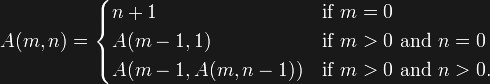
Today we return to to the topic of mathematics with a look at Ackermann’s Function. Anyone who has studied computer science has probably encountered this function (though I’m sure many have gone on to forget it). It is most commonly defined as follows:

This is actually a variant of Wilhelm Ackermann’s original function, often called the Ackermann–Péter function. It is quite a simple function to define and to trace, and it is very easy to implement in just about any programming language, including Python:

def ackermann(m, n):
  if m == 0:
    return n + 1
  elif n == 0:
    return ackermann(m - 1, 1)
  else:
    return ackermann(m - 1, ackermann(m, n - 1))

However, its complexity (in terms of run-time and memory) grows quite quickly. As such, it is often used as an exercise in teaching students more complex forms of recursion, and also as a test case in compiler development for optimizing recursion. It also has some interesting mathematical properties for particular values of m:

The numbers in the case of A(4,n) are quite large. Indeed, one could describe Ackermann’s function as “computing really really large numbers really really slowly.” Although the numbers grow quickly, the function is really just doing subtraction and recursion. We can take advantage of the properties described above, however, to make some shortcuts that yield a much more efficient function.

def ackermann(m, n):
  while m >= 4:
    if n == 0:
      n = 1
    else:
      n = ackermann(m, n - 1)
    m -= 1
  if m == 3:
    return 2 ** ( n + 3) - 3
  elif m == 2:
    return 2 * n + 3
  elif m == 1:
    return n + 2
  else: # m == 0
    return n + 1

With this version computing A(m,n) for m≤3 becomes trivial. And this makes computations for m≥4 possible. Or at least A(4,2), which we can actually run in python to reveal the 19,000 digit answer.

You can see the full value on this page. Computing A(4,3) is infeasible. Even with the optimizations, most computers will run out of memory trying to compute this value. But one can still reason about these rather large numbers. Let us move from the more common function we have been using to Ackermann’s original version:

This version has three arguments instead of two, and on the surface it may seem a bit more complicated. However, different values of the third argument p yield very familiar operations.


Again, this function is a rather inefficient way to compute addition, multiplication and exponentiation, but it is an interesting way to reason about them and extrapolate to other more exotic operations. For example, if we take p to be 3, we get the following operation.

Just as m x n is adding m to itself n times, and exponentiation mn is multiplying m by itself n times, this new operation (sometimes called tetration) is the next level: exponentiating m by itself n times.

Such an operation grows so fast as to be uncomparable to exponential growth. It grows even too fast to compare to the gamma function which have explored on CatSynth in the past. This series of ever higher-order operations is often noted with an arrow, called Knuth’s up-arrow notation after legendary computer scientist Donald Knuth.

Using this notation, we can define as sequence of numbers, called Akermann Numbers, where each is an ever higher-order operation of the element applied to itself.

  • 1↑1 = 11 = 1,
  • 2↑↑2 = 2↑2 = 22 = 4,
  • 3↑↑↑3 = 3↑↑3↑↑3 = 3↑↑(3↑3↑3) = 

Even just the 4th number is this sequence is so large that we can’t even easily notate it with exponents. So forget about the 5th number in sequence. But a question that interests me is what about interpolating with real numbers. What is the 1 1/2th Ackermann number? That question, if it even has an answer, will have to wait for another time.

Weekend Cat Blogging and Photo Hunt: Heart

Our combined Weekend Cat Blogging and Saturday Photo Hunt features the theme Heart. We have a few images that blend the theme with our interests in music, mathematics and of course, cats.

Here Luna poses with a heart-shaped kalimba (thumb piano).

Luna peers at the iPad, which displays a plot of a cardioid. We used a mathematical function that produces the heart-shaped figure when plotted with polar coordinates. The formula for the cardioid is: r = 1 – sin(θ), where r is the radius from the center of the plot and θ is the angle sweeping around the center. The best way to visualize polar coordinates is using one of those old circular radar screens where the plotter sweeps in a circular motion.

The photo also features one of Luna’s favorite toys, a heart-shaped plush toy with the word “kitty” inscribed on it. We have had it for years now (indeed, it was featured in a WCB/Photo Hunt back in 2008).


Weekend Cat Blogging #349 (Valentines Day edition) is hosted by Meowza.

The Saturday Photohunt theme is Heart.

The Carnival of the Cats will be up this Sunday at Meowzings of an Opinionated Pussycat.

And the Friday Ark is at the modulator.

11:11 on 11/11/11

At 11:11 on this day 11/11/11, I snapped screenshots of both the iPad and iPhone featuring Luna.

Of course, the symmetry and homogeneity of the date and time is quite attractive, and unique (at least within a given century). The number 111111 is also interesting when you decompose it into primes:

111111 = 11 * 13 * 3 * 37 * 7

I find the prime factorization quite poetic.

We can also factor the date and time together (11:11:11 on 11/11/11):

111111111111 = 11 * 13 * 3 * 37 * 7 * 101 * 9901

Note quite as poetic as the previous example, but still interesting. In particular, 9901 is interesting as the greatest prime factor for any repeating series of 12 numbers. Other related properties can be seen at the site Prime Curios.

Weekend Cat Blogging and Photo Hunt: Digital

The theme of this week’s Photo Hunt is digital. Rather than simply use a digital photo – which could be any photo ever taken of Luna – I chose a couple of images that demonstrate the unique opportunities of the medium. A digital photo is really just a stream of numbers, not unlike digital audio, and can be processed in countless ways using digital signal processing or applying other mathematical functions.

For a piece I originally did in 2007, I took one of Luna’s adoption photos from Santa Cruz County Animal Services and applied an algorithm that overlaid these colored bands, as shown above.  The color bands were generated using a set of hastily chosen trigonometric and hyperbolic functions applied to the timeline of the animation sequence.  These photos are stills from the full animation.

I did these using image and video extensions to Open Sound World – one nice feature of that work was that I could use the same functions for both audio and video, and “see” what a particular audio-processing algorithm looked like when applied to an image.   And I would probably use the Processing environment for future visual work, perhaps in conjunction with OSW.


Weekend Cat Blogging #309 and Carnival of the Cats are both being hosted by Billy SweetFeets this weekend. Perhaps Luna’s animation could be part of one of the dance videos they often feature.

Photo Hunt #264 is hosted by tnchick. This week’s theme is digital.

And the Friday Ark is at the modulator.

A special note this week. Our friend Judi at Judi’s Mind over Matter (home of Jules and Vincent) has information on how to help animals affected the storms and tornadoes in the southeast US. They live in Alabama, not far from the place that was hit hardest by the tornadoes. We’re glad they’re safe, and able to provide this information for those who would like to help.

108

Sometimes when things get a bit overwhelming it’s good to turn to numbers and highways. As mentioned in earlier posts, I maintain a rather cursory yoga routine for both health/exercise and grounding. The number 108 comes up fairly often in cycles of repetition and I have been curious about its significance. Long before it was featured on Lost, 108 prominently figured in Hinduism as the number of beads on a mala and in other contexts, and through Hinduism finds its way into Buddhism. 108 has several interesting purely mathematical properties. My favorite is its being the hyperfactorial of 3. The hyperfactorial is the product of consecutive integers, each raised to itself as an exponent:

11 x 22 x 33 = 108

Among the more random properties is being the sum of 9 consecutive integers:

8 + 9 + 10 + 11 + 12 + 13 + 14 + 15 + 16 = 108

9 is of course a divisor of 108, as in 9 x 12 = 108. And both 9 and 12 appear in the above series.

More significantly, 108 degrees is the angle of a vertex a regular pentagon, and 108 degrees can also be used to derive the golden ratio.

The relationship to the golden ratio would seem to be an interesting one, until one remembers that the representation of angles as degrees is itself arbitrarily based on the number 360. The 3π/5 radian representation is more significant in this regard.

And what about fun with highways numbered 108? Here in California, state highway 108 runs from the Central Valley town of Modesto northward and eastward across the Sierra via the Sonora Pass (north of Yosemite) to meet US 395 on the eastern side of the Sierra.

[Photo by jodastephen on flickr.  (License CC BY-ND 2.0)]

While I have not driven CA 108, I am sure I have crossed its path on CA 120 on the way to Yosemite. From the picture above, it looks like it would be a nice drive, particularly in the summer. The eastern side of the Sierra has that stark, desolate quality, in comparison to the heavily wooded slopes on the western side. They are both quite beautiful, but the eastern side tends to speak to me more.

In New York, Route 108 is a short highway on Long Island. In fact, it is very short, a little under two miles total.  It’s southern terminus is the picture below.

[Photo by dougtone on flickr.  (License CC BY-SA 2.0)]

Route 108 southbound crosses into Nassau County, but soon curves away back into Suffolk. Soon after, the two-lane road continues into Trail View State Park, where the route becomes desolate, passing two local ponds.

It is interesting how the word “desolate” can come up for both highways, with very different connotations.

Pi Day, 2011 (with Music)

Every year, we at CatSynth join numerous other mathematics enthusiasts, geeks and otherwise eccentric characters in celebrating Pi Day on March 14.

March 14 is notated in the U.S. and some other countries as “3-14”, which evokes the opening digits of π (pi). Although the date representation is a very arbitrary connection to the number, we also recognize that the representation of π in decimal digits is arbitrary, an accident of human beings having ten fingers. So this year we are exploring the representations in binary and other related bases.

To represent an integer in binary, one of course presents it as a sum of powers of two, e.g., 11 = 8 + 2 + 1 or 1011 in binary. But one can also represent fractional numbers in binary. Digits to the right of the decimal point represents powers of one-half. So the binary number 0.11 is 1/2 + 1/4, or 3/4. Fractions like 1/3 can be represented with repeating digits as 0.010101…, much like in base ten. And this concept can be extended to irrational numbers like π.

The author of this website has calculated 32768 digits of pi in binary. We reprint the first 258 below:

11.
00100100 00111111 01101010 10001000 10000101 10100011 00001000 11010011 
00010011 00011001 10001010 00101110 00000011 01110000 01110011 01000100 
10100100 00001001 00111000 00100010 00101001 10011111 00110001 11010000  
00001000 00101110 11111010 10011000 11101100 01001110 01101100 10001001 

The initial “11” represents the 3 in π, and the remaining digits begin the non-integral portion. Like in the decimal representation, the binary representation continues forever with no particular pattern. While not as iconic or memorable as the decimal representation 3.14159…, there is something about the binary representation that makes it seem more universal, i.e., based on fundamental mathematical truths rather than a quirk of human anatomy. For me, the binary representation also lends itself to musical ideas. And for the occasion, I have created a couple of short synthesized pieces representing the 32768 binary digits of pi. In the first example, each binary digit represents a sample. The “1” represents full amplitude and the zero represents no amplitude (silence). The result, which at 44.1kHz sample rate is less than one second long, can be heard below.

The random configuration of digits sounds like noise, and more specifically like white noise, suggesting something approaching uniform randomness at least to human hearing. I also made an example slowed down to a level whether the individual samples became musical events. I find this one quite interesting.

With some additional refinement (and may some more digits to extend the length), it could certainly stand alone as a composition.

One interesting counterpoint to the notion that digits of pi form white noise is a conjecture related to its representation in hexadecimal (base 16), which as a power of two is “closer” to binary and seemingly less arbitrary than decimal. From Wolfram MathWorld, we find the following “remarkable recursive formula conjectured to give the nth hexadecimal digit of π – 3 is given by where is the floor function:

The formula is attributed to (Borwein and Bailey 2003, Ch. 4; Bailey et al. 2007, pp. 22-23). If true, it would add some sense of order to the digits, and thus additional musical possibilities.